How To Use Graphviz for SEM Models and Path Diagrams
Graphviz is a free graph
visualisation program that produces structural diagrams. While its primary
purpose is visualization of algorithms and flow charts, it can also be used
to draw path diagrams and structural equation models. The syntax resembles
somewhat that of R's
sem package: it uses the same idea of -> signs
to represent the arrows. The variables of the model are nodes in
Graphviz slang, and the relations are edges.
Example 1: Holzinger-Swineford CFA model
Holzinger and Swineford data and model is one of the favorite
toy data sets in confirmatory factor analysis popularized by
Joreskog (1969)
and used as an example in
Yuan and Bentler (2007). The data set itself is available
here
with SPSS syntax, here as Stata dta file,
as well as in R package MBESS.
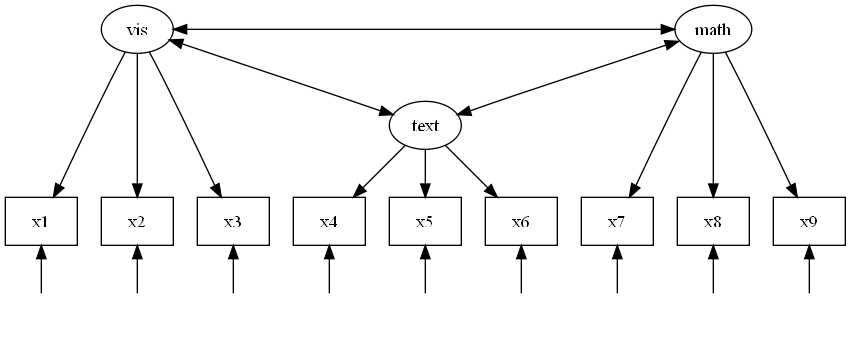
The path diagram associated with this model can be produced
in Graphviz as follows:
Here's the code that produces this graph using Graphviz' dot engine.
digraph HSCFA {

   vis -> x1 [weight=1000];

   vis -> x2 [weight=1000];

   vis -> x3 [weight=1000];

   text -> x4 [weight=1000];

   text -> x5 [weight=1000];

   text -> x6 [weight=1000];

   math -> x7 [weight=1000];

   math -> x8 [weight=1000];

   math -> x9 [weight=1000];

   vis -> math [dir=both];

   vis -> text [dir=both];

   text -> math [dir=both];


   x1 [shape=box,group="obsvar"];

   x2 [shape=box,group="obsvar"];

   x3 [shape=box,group="obsvar"];

   x4 [shape=box,group="obsvar"];

   x5 [shape=box,group="obsvar"];

   x6 [shape=box,group="obsvar"];

   x7 [shape=box,group="obsvar"];

   x8 [shape=box,group="obsvar"];

   x9 [shape=box,group="obsvar"];


   { rank = same; x1; x2; x3; x4; x5; x6; x7; x8; x9 }

   { rank = same; vis; math; }

   { rank = max; d1; d2; d3; d4; d5; d6; d7; d8; d9 }


   d1 -> x1;

   d1 [shape=plaintext,label=""];

   d2 -> x2;

   d2 [shape=plaintext,label=""];

   d3 -> x3;

   d3 [shape=plaintext,label=""];

   d4 -> x4;

   d4 [shape=plaintext,label=""];

   d5 -> x5;

   d5 [shape=plaintext,label=""];

   d6 -> x6;

   d6 [shape=plaintext,label=""];

   d7 -> x7;

   d7 [shape=plaintext,label=""];

   d8 -> x8;

   d8 [shape=plaintext,label=""];

   d9 -> x9;

   d9 [shape=plaintext,label=""];


}
You can try to figure out how stuff works by commenting
a line out with C-style comments // and running Graphviz again.
Let us go over this code and learn some tricks.
- digraph is the keyword that introduces a directed graph.
- Lines 2--13 introduce the relations between the latent variables
vis (visual factor), text (reading analysis factor)
and math (counting factor), as well as their relation
to the observed variables x1 through x9.
- weight=# option gives some degree of control
over the shape of the line. The greater the weight, the
more straight and the shorter the line becomes. 1000 is a
really big number, so the lines must come as straight as possible.
- The option dir=both requests a two-sided arrow.
- Lines 15--23 specify that the observed variables be put in boxes
rather than default ovals. The group keyword
indicates that these nodes belong to the same group,
and should be layed out at the same level of the diagram.
- rank=same; followed by the list of variables
additionally forces placement of all the variables at the same
level.
- rank=max; followed by the list of variables
forces those variables to appear at the very bottom of the diagram.
- The desription of the error terms d1--d9
generates the upward arrows. Generally Graphviz thinks
about directed graphs as flows that go in a certain direction
(from left to right and from top to bottom), so these arrows
are going against the flow. Hence we need to force the origins
of these arrows to be below their respective x1--x9
variables with rank=max; command just discussed.
- shape=plaintext option requests that a node
is displayed without any contours around it, so that a label
is reproduced as is.
- label="" requests that a label for this node is empty.
The joint effect is that nothing at all is produced
in place of d1--d9 variables.
It is more customary in the SEM literature to denote the covariances
by curved two-sided arrows. Graphs like that can be forced through
Graphviz, but their aesthetic appeal is probably not that great:
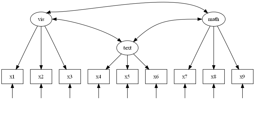
The change that's needed for this graph is to replace the
relations between the factors by
   vis:ne -> math:nw [dir=both];

   vis:e -> text:nw [dir=both];

   text:ne -> math:w [dir=both];
The specification node:position in place of node
attaches the arrow at the given compass position.
It forces some curvature into the lines, although there is no
other control over the shape of the line.
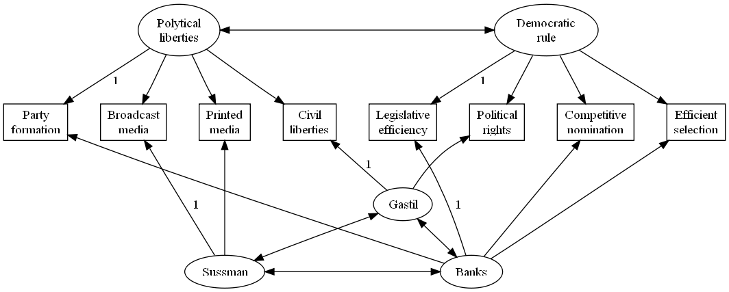
Example 2: Bollen's liberal democracy model
Bollen (1993)
builds a multiple traits - multiple methods (MTMM) model
of liberal democracy. There are two main factors,
or traits (polytical liberty and democractic rule),
and three methods factors (sources of data, political science
researchers A. Banks, R. D. Gastil, and L. R. Sussman).
The path diagram is as follows (the individual error terms
are omitted):
Self-check: produce the above diagram using Graphviz.
Hints: multiple line lables are produced by inserting
the C-style end-of-line character "\n", and the fixed
loadings are produced with label option.
© Stas Kolenikov, 2009.