xstata
or
stata
at the command prompt to start a graphic or text interface of Stata.
To start Stata, locate Stata icon ![]() on your desktop, or go to
Start -> Programs -> Stata (it may be Stata 8, Small Stata, Intercooled Stata 8, or something
else that does have a word "Stata" in it!). On UNIX machines, type
on your desktop, or go to
Start -> Programs -> Stata (it may be Stata 8, Small Stata, Intercooled Stata 8, or something
else that does have a word "Stata" in it!). On UNIX machines, type
xstata
or
stata
at the command prompt to start a graphic or text interface of Stata.
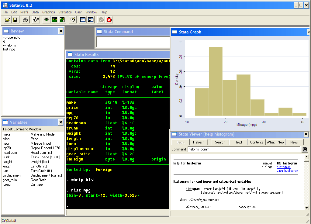
Click on different areas of the above picture to see a short description of the area.
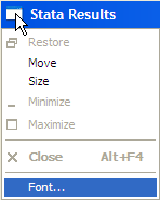
You can change the font in a specific windows by left-clicking at the top left corner
of the window where the font is to be changed.
To exit Stata, type
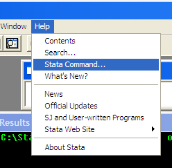
To find a help on a command you already know, go to Help menu -> Command:
All of the Stata help files are duplicated on the web.
Stata Interface
. exit
in the command prompt, or click the X-button at the top right corner, or double-click the
top left corner icon ![]() . If there are any unsaved data, Stata will
resist exiting.
. If there are any unsaved data, Stata will
resist exiting.
Help and Search
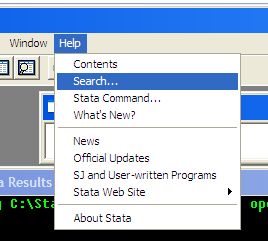
To search for a concept, go to Help menu -> Search:
. search linear regression
in the command prompt. By default, search goes over the built-in
help files available locally on your machine. If you want to also search over
the Internet (which will bring you some goodies from other Stata users as well), enter
search phrase, all
or
findit phrase
. help regress
in the command prompt for the help file to show in the Results window, or
. whelp regress
for the help file to show in the Viewer window (more convenient).
| Self Check:
|
Stata has a somewhat idiosyncratic system of references to its manuals. In the bottom of pretty much every help file you'll see something like this:

More on working directories later, with the discussion of the do-files.
Do you still remember?..
Make sure you keep the log of what you are doing! Stata has two sorts of logs:
Advice: open a command log in the startup script, and open / close a log file in every do-file you write.
More on that later.
command [variable(s)] [if expression ] [in obs. range
] [[weights]] [using filename], [options]
The command is performed on the variables if applicable, a particular
subset of observations may be selected by the if and in modifiers, and the specific
ways the command should behave are controlled by options. The most complex and powerful
commands may have several dozen different options.
See also a note at UCLA Academic Technologies
Services Stata website.
You can usually figure out how much memory Stata may need by looking at the sizes
of the data files you are planning to work with. You can do that by typing
There is also a neat trick of loading only the data you need. Recalling the general syntax
of a Stata command, you might try
Another trick you might want to explore is to take a subsample of your data with
See also UCLA Academic Technologies
Services Stata web site.
Sometimes, the raw data comes in a plain text format, either
a fixed format (where the data from a particular column should
form a variable), or comma/tab separated format (where the data for a
single observation are listed in a line and are separated by a comma or
a tab character). Such data can be read into Stata by
See more extensive description at
UCLA Academic Technologies Services web site.
From Stata, you can also save the data into a text file (to be exported to other
applications):
Stata comes with a bunch of toy data sets that are often used for educational purposes. You
can retrieve the list of those data set by
. log using filename
to copy everything that goes to the Results window into a specified file, and
. cmdlog using filename
to copy the commands only (useful for converting an interactive session into a do-file; more on do-files
later). See help log
for useful options replace, append, and formats smcl
(hyper-referenced) and text (plain text)! You can also use the streetlight button
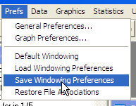
on the toolbar menu to control the log flow. The status bar at the bottom of the Results window
shows the current log status.

. log close
but Stata will close the file when you exit automatically.
Generally speaking...
Most Stata commands have the following syntax:
Loading data
Stata has its own format of data files. Stata data files have extension .dta. To load
a data file into memory, type
. use auto
Stata will look for the file named auto.dta in the current directory.
In fact, this is a file that comes with the distribution of Stata
and is available in Stata system directory. Try this out:
. sysuse auto
use is a more versatile command that it may seem, as it allows loading a portion of the
data set with if and in modifiers (more on that later), as well as loading
the data over the Internet:
. use http://wps.aw.com/wps/media/objects/284/291498/caschool.dta
You can come across some errors while loading the data. Stata will show error messages
in red, and the typical messages will be:
no; data in memory would be lost
You tried to load the data on top of the existing data files that was not saved. If you are
sure you want to lose the changes you made to your current data, type
. clear
to clear the memory, or specify use ..., clear option.
no room to add more observations
Stata did not have enough memory to load all of the observations. The next few lines
give some suggestions on how to proceed, and the most important one is how to set the amount
of the memory that Stata should request from the operating system.
Memory issues
To see how much memory Stata uses now, and how this memory is being used, type
. memory
To change the amount of memory Stata can address, type
. set memory 40m
to request 40 Mbytes of memory.
. ls
or better
. ls *.dta
to request a listing of dta-files.
Stata also needs some overhead for programs and temporary objects; most of the time,
adding some 15-25% is enough. Keep in mind however that when the amount of memory reaches
the physical memory of a computer (256 or 512 Mbytes on contemporary PCs), it begins swapping
the data into a temporary files on the hard disk, and the operation slows down by a factor of
about 100 to 1000. (This is not Stata's fault, this is the way virtual memory is organized
in Windows. UNIX operation is usually much smoother.)
use varlist if exp using filename
to load only those observations and variables you actually need. It does save you
a lot of trouble.
sample #, [count]
and design your analysis with this subsample. Once you have a clear plan of what you would
want to do, write a do-file (i.e., a sequence of Stata commands that can be run from
within Stata) and leave it overnight, or over weekend... or over vacation if you are
going to have any at all :).
Saving your data
To save the data, type
. save filename
You might need to specify save ..., replace option if the specified file
already exists. USE WITH CAUTION! You certainly must have your original data
in a safe place, and be sure not to ever, ever overwrite it.
Converting the data from other formats
Unfortunately, Stata cannot read formats other than its own .dta or text files.
However, you can nicely convert the data between different formats by the third party utilities
such as StatTransfer or
DBMS/COPY.
It supposedly works with SAS XPT files (see
fdause), but I've never tried it.
. infile variables using filename, [clear]
This is also the way to export data from Excel: the data should be saved
as a plain text (comma-separated format, csv), and then they can be read
into Stata by infile or infix.
. outfile [variables using] filename, [replace]
. sysuse dir
and load the most popular data set on a few cars and their characteristics by
. sysuse auto
Looking at the data
Let us
. sysuse auto
to begin our session with the data. What kind of data is there? Type
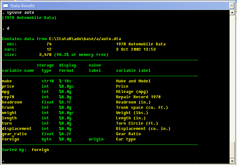
. describe
to get an overall picture. In fact, it suffices to type
. d
for Stata to recognize that this is an abbreviation of describe. We shall denote the minimal
abbreviation by underlining it:
. describe
Aside: Stata colors
Aside: Stata guts: storage types
One important piece of information we can take from the above description of the data set
are the storage types of the variables in the data set. Stata distinguishes discrete,
floating point (roughly speaking, continuous) and string data types. Within each of those
types, there are also distinctions by the range of the values and accuracy. Most importantly,
for many applications the accuracy of the float type is insufficient, and it is a good
idea to use double precision in your data files and programs.

| Self Check:
Which of the following will produce an accurate answer, and which one will not?
|
Note that rep78 variable has a few missing values. We'll see how this may be of importance
in data handling and analysis.
Back to looking at data
Can we have a sneak preview on what is in there? Folks who are more used to a command line would type
. list
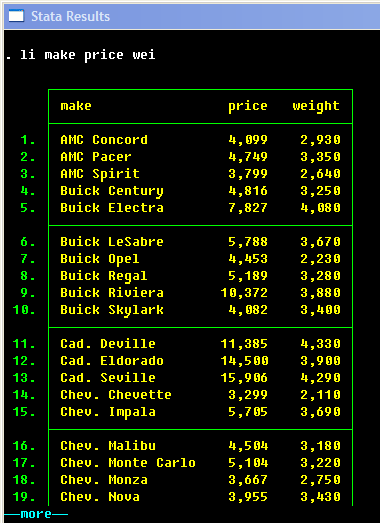
to get a listing of existing variables and observations. Note the --more--
thing in the bottom: you need to hit Enter for the next line, and hit Space or click this
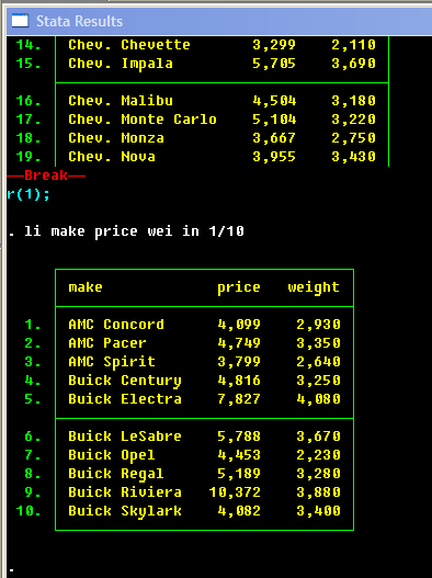
--more-- condition for the next screen. Press Q or Ctrl+C or Ctrl+Break (Windows)
or hit the Break button  .
Looks like too much information, huh?
Try this:
. li make price wei
. li make price wei in 1/10
. li m

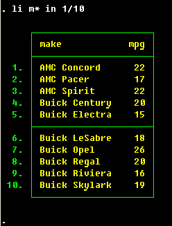
| Self Check:
How many variables are there in each of the following varlists?
|
Another way to select specific observations is by if qualifier. It takes a form
if logical expression.
A logical expression is an expression that can be either true or false, and usually it constitutes
a comparison of two numeric expressions. If it sounds too complicated, consider this:
. li make mpg pri if mpg>25
Here is the notation for the available comparison operators. Note the notation for the
equality comparison. We shall see a bit later that the single equal sign, =, is used
for assigning the values to new variables, specifying weights, in some cycle operators, etc.,
while the double equal sign introduced now is used exclusively in the if expressions.
| Symbol | Meaning |
| > | Strictly greater |
| < | Strictly less |
| >= | Greater or equal |
| <= | Less or equal |
| == | Equal |
| != or ~= | Not equal |
Logical expressions can be combined:
. li make mpg pri if mpg>25 & weight > 2500
The logical operations that can be performed are logical AND (the result is true
only if both arguments are true; denoted in Stata by &), logical OR (the result
is true if any of the arguments is true; denoted in Stata by |), and logical NOT
(works on a single argument changing true to false, and vice versa; denoted in Stata by ~
or by !).
Small print (but still useful to know): in fact, Stata uses numeric values for true and false, and that again comes from C++ programming language (where, in turn, it reflects the basic electric impulses the computer operates with). Logical true is denoted by 1, and logical false, by 0. So with those numeric values, we can set up a table that shows the results of logical operations.
|
||||||||||
| OR: | | 0 | 1 | ||||||||
| 0 | 0 | 1 | ||||||||
| 1 | 1 | 1 |
| NOT: ~ or ! | |
| 0 | 1 |
| 1 | 0 |
Even smaller print: in fact, Stata can interpret any numeric expression
as a logical (true/false) one. If an expression evaluates to zero, then Stata takes
it as a "false"; if it is a non-zero, Stata takes it as a "true". Here's an important catch:
if expression evaluates to missing, it is still not zero, and Stata takes it as a "true".
Also, as long as the missing values are greater than any number, "greater" and "greater or
equal" comparisons select missing observations, too.
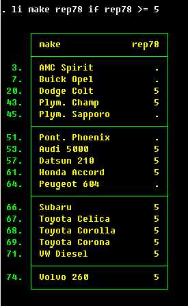
Hence, in all of your comparison commands you might to explicitly filter for the
missing values with a function mi(exp) that returns 1 when
the exp evaluates to missing, and zero otherwise. Compare the results of
. li make rep78 if rep78 >= 5
and
. li make rep78 if rep78 >= 5 & !mi(rep78)
| Self Check:
|
 |
Stata is very fast when
it needs to perform an operation on the whole column (such as creating a new variable,
which we'll do in a second, or running a regression that uses several variables -- which, as
you would recognize, involve some matrix operations), and it is painfully slow when you
instruct Stata to do operations on single observations by in 1, in 2, etc.
manner. It is never a good idea to do the latter unless it is absolutely inevitable. Most of the
time, there should be a trick or two to do what you need!
Stata's command for sorting is sort. Have a look through this sequence:
Small print: what will Stata do if the values of the sorting variable are not unique?
Sorting the data
For many operations, like computing the means or running a regression, the sort order of
the data is pretty much irrelevant. There are occasions, however, where you do want one
observation to follow another in a strict order. An obvious example is time series data,
where the sort ordering is simply by time. Other, somewhat less obvious examples, might be
panel data, where you would want to have observations pertaining to the same individual, but
differing in time, to be next to each other; or welfare distribution analysis, where measures
like poverty indices or Gini coefficient of inequality require sorting by income (or another
welfare measure).
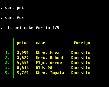
. li pri make for in 1/5
. sort price
. li pri make for in 1/5
. sort for make
. li pri make for in 1/5
sort sorts the data sequentially in the ascending order by the first variable specified, then
within the range of the same values of the first variable, by the second variable, etc.
If you need a descending order, the command you would want to use is gsort. If you need
to order the variables in the Variable window, use aorder to order the variables
alphabetically, or order to move specific variables to the front.
Summary statistics
OK, we now know how to have a look at the data set. Can we get a more condensed summary
of information contained in it? Here you go:
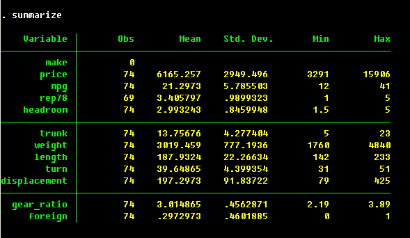
summarize is a fairly powerful command.
It can take variable lists and if/in qualifiers with it. And it can do much
more with detail option; see
UCLA Academic Technologies Services Stata website.
| Self Check:
|
So, means, medians and such are measures for a single variable. What might we be interested for
two variables? Of course, a correlation:
If we look at the help file for correlate, we shall find a number of suggestions
at the bottom (you will always find something under See also section of the help file,
but now I'd like to draw your attention to it) to look at the pwcorr command. Unlike
correlate that first restricts the data set for the non-missing observations, and then
computes those correlations (available case scenario), pwcorr computes correlations
for maximum number of available observations for each pair (pairwise scenario). Compare
You can ask pwcorr to tell you how many observations it is used, and test the null
hypothesis of zero correlation, by specifying obs and sig options, respectively.
See some more details at
UCLA Academic Technologies Services Stata website.
. correlate wei len
Is it reasonable to think that longer vehicles are heavier? It looks so, at least judging
by the sign and the magnitude of the correlation coefficient.
corr rep78 wei len
and
pwcorr rep78 wei len
| Self Check:
|
You can find everything you need about Stata graphics from the help file graph.
Type
. whelp graph
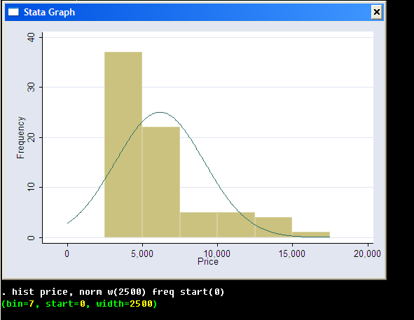
... and see how easily one can get lost in it. Histograms are not even mentioned there,
but if you search histogram or just make an educated guess, you'd find histogram
command to perform what you would need:
| Self Check:
|
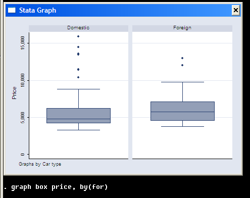
| Self Check: Make a side-by-side box-plots of car prices for different values of the repair record variable. Are there any notable differences in prices? |
Other, sometimes interesting and valuable, summaries are provided by inspect and lv
commands.
There is more versatility to those graphic commands, however, and a much nicer plot may be produced
as this:
Scatter plots
For two variables, one of the best graphical summaries is a scatter plot:
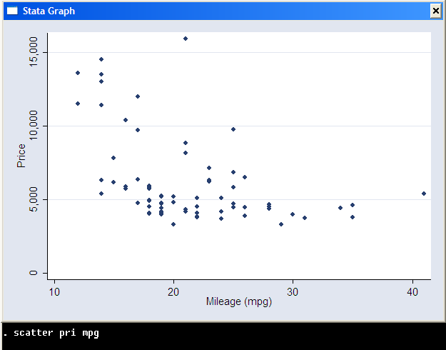
. scatter pri mpg , by(for)
and that is a legal syntax to do (try it now!).
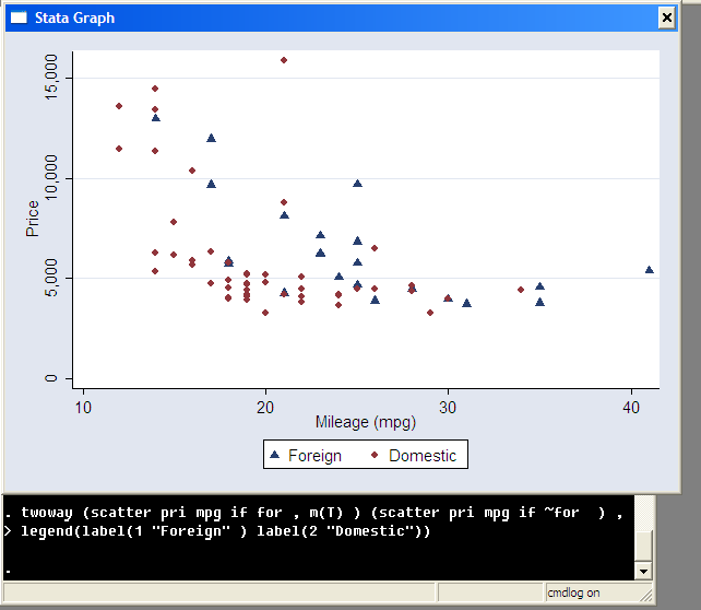
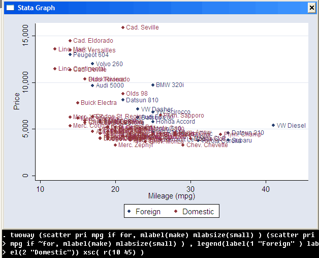
One of the nice twists you can make to your graphs is to put some identifying information by the side of the observation. This is done by mlabel(variable) option; mlabsize() control the size of the graph. xsc() makes sure there is enough space in the left side of the graph for the most economic Volkswagen on the roster.
Let us stop here and review again what we've learnt in this tutorial.
On to the next class, to learn about the ways of modifying the data and some Stata-special tricks to quickly solve seemingly difficult data management problems.
Questions, comments? E-mail me!.
Stas Kolenikov