Class 3: Estimation

In the previous classes 1 and 2 we learned some basic things about Stata:

Stata's interface and help system
Logging one's Stata sessions
Reading the data into Stata
Looking at the data
Getting basic statistical summaries and making basic statistical graphs
Specifying specific sets of observations for a Stata command to work on
Developing an understanding of the numeric accuracy and missing values
Creating new variables and changing the existing ones
Using Stata functions
Using subscripting variables _n, _N
Using by: construct

In this class, we shall get a hold on the basics of Stata estimation commands. Automobile data will be used as an example of data, and regress will be used to demonstrate the main features of many estimation and post-estimation commands. We'll only have major differences for systems of equations such as those in simultaneous equations or Heckman model. Panel, time-series, or survey data will only differ in the amount of time one would need to spend setting up the data for estimation.

All of the estimation commands feature the same overall approach. You need to specify the dependent variable, the explanatory variables (if any), the subsample (if/in) and some estimating options (such as corrections for heteroskedasticity or clustering, maximum likelihood convergence criteria, twostep vs. FIML estimation in Heckman model, etc.). Stata gives you the estimation output where you can check the basic results such as overall significance, and significance of individual explanatory variables. After estimation, you can test linear and nonlinear hypothesis or estimate linear and nonlinear combinations, and get predicted values, predicted probabilities, residuals, and some other observation-level statistics. The results of the estimation are stored in Stata memory until the next estimation command, or until erased explicitly.

OK, let's start:
. cd your favorite location . log using class3, replace . sysuse auto

Linear regression

Linear regression is a standard starting point in many analyses (although it really is a starting point, as the analysis usually moves much beyond the scope of this simple model pretty fast). As we found out in the first class, the Stata command to perform a linear regression is regress. It deserves putting up its full syntax here. Click here to open it in a separate window. Let us go slowly through it exemplifying the concepts as we go.

The basic part of the syntax is
. regress depvar[ varlist]
which means a regression where the dependent variable is depvar, and the list of regressors is in varlist. Let's try it off:
. reg pri mpg wei for

In the upper left corner of regression output is the ANOVA table, i.e., a decomposition of the total sum of squares of the dependent variable. If you don't have a clue about ANOVA, you can leave it at that; it can be mentioned that the R² is computed as the ratio of the Model SS to the Total SS. On the right, there are overall summaries of the regression: the number of observations, the F-test for the overall significance, R² and adjusted R²_adj, and the square root mean squared error of the residuals.

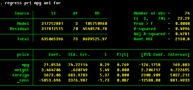
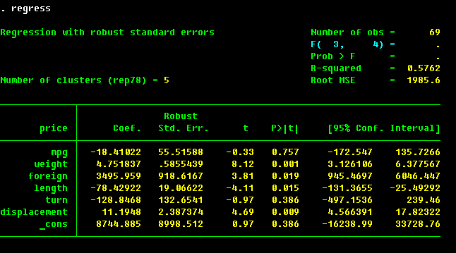
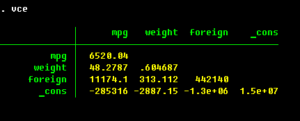
The most important information is in the lower pane of the regression output. Here we have the names of the dependent variable (price) and of the explanatory variables (mpg, weight, foreign; _cons is the constant term, or the intercept of the regression. To omit one, specify nocons option of regress. To indicate to Stata that you already have a constant term among regressors (this is helpful in some panel data regressions), specify hascons option). The next column are the estimated coefficients β = (X^TX)^-1X^TY. The third column are the estimated standard errors, which are the square roots of the diagonal entries of the estimated covariance matrix, which in this is s² (X^TX)^-1 (it is going to be different for some other models). The t statistics in the next column are the ones to test the null hypothesis of no linear relation between the explanatory and the dependent variable conditional on other explanatory variables (i.e., that respective β is equal to zero). The p-value for the test is provided in the next column. Finally, the confidence interval for the coefficient is given in the last two columns.

A little bit longer explanation of what Stata shows after regress is available at UCLA Academic Technologies Services Stata website.

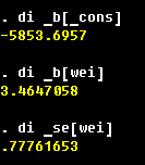
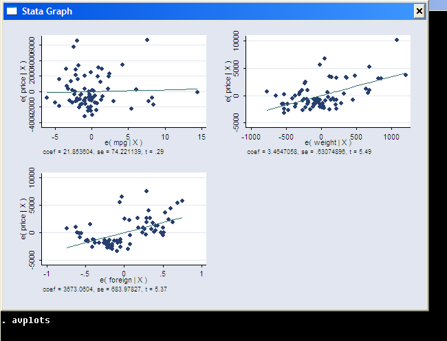
From the estimation results, we can infer that weight and price are positively related, that the foreign cars are on average more expensive by $3673, and the mileage is not significantly related to price in this model. The R² is reasonable at 0.50, but not particularly high. Let us refer to this model as Model 1. We can save the estimation results in Stata, too:
. estimates store Model1

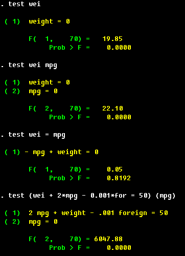
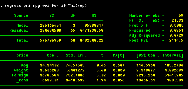
As with most Stata commands (and as with all estimation commands), you can add if/in qualifiers to restrict the estimation subsample:

This will be Model 2. A linear regression model is overly simplistic and very limited, and you as a researcher should get a feeling of whether it is appropriate or not. The minimal thing to do (and it is very easy to do in Stata) is to correct the covariance matrix of the estimates for heteroskedasticity (non-constant variance). Economists know this correction as White estimator; statisticians, as Huber estimator; survey researchers, as linearization estimator; other names it goes under are robust estimator (although an argument can be raised against this term since the meaning of robust methods is somewhat different in the classic texts on robust statistics), and sandwich estimator (which is probably the most appropriate and neutral; the name is such since the analytic form of this estimator does resemble a sandwich of several matrices). The option is robust:

Let us call this Model 3:
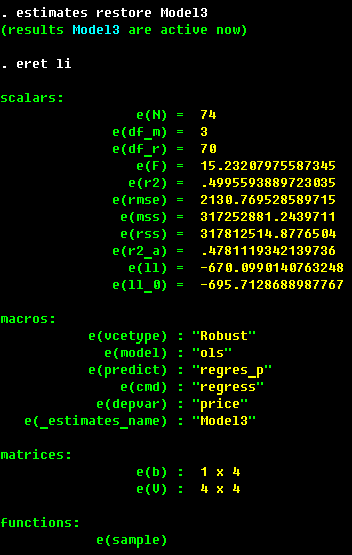
. estimates store Model3
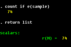
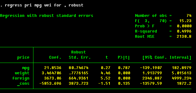
Note that we have the same subsample as in Model 1. The point estimates are the same, but the standard errors are slightly larger, except for foreign variable. This increase is a typical outcome of the correction.

In general, the robust correction is available for most models estimated by maximum likelihood; see help for _robust. Linear regression is an example of such model if one assumes normality of residuals. The robust correction in this case gives consistent estimates of the standard errors if the distribution of the residuals is different from the normal with fixed parameters. For models such as probit, the corrections is for the violations of the assumed probability distribution (say the underlying link between Xβ and the probability of a positive outcome is logit rather than probit).

If you have reasons to believe that some observations are grouped together by the data generating mechanism, you can specify cluster() option to account for this effect:

Let this be Model 4. Note that the estimation subsample was restricted to the observations where rep78 is not missing, so the point estimates are identical to those of Model 2. Some of the standard errors, however, have increased substantially, almost by the factor of two, due to clustering. This is usually suggestive that observations within clusters have similar values of the corresponding variable. Note also that Stata mentioned that there were 5 cluster according to the unique values of rep78. If we had more regressors than the number of clusters, Stata would run out of degrees of freedom to assess the overall significance:

The models where the number of clusters is less than the number of explanatory variables produce singular cluster-corrected covariance matrices of the coefficient estimates. This is not as drastic as under-identification of a linear regression model if you have fewer observations than explanatory variables, but it still is a rather unpleasant effect. For instance, it means that some combinations of the coefficient estimates would have zero estimated variance, the effect similar to collinearity among regressors.

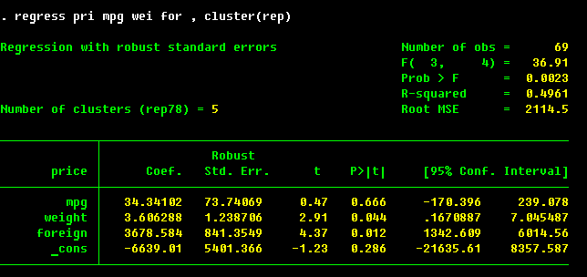
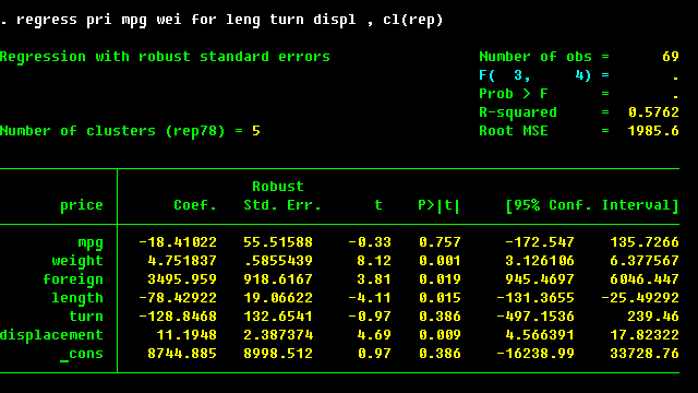
The correction for clustering is a must for survey data where the clustering reflects the multi-stage sampling design. The correction to be made then is for clustering at the very first level of sampling.

Self Check: Run the regression of mpg on weight, foreign and length. Do the results conform to your expectation? What is the R² of the model? Which variables are significant?

Post-estimation commands

Saved results

As was mentioned before, Stata saves estimation results in its memory between two estimation commands. One can retrieve the results in their original form by re-typing the estimation command again:

In this case, the last estimated model was the one with insufficient number of clusters (or rather excessive number of variables). Let us fall back to Model 3 with "robust" standard errors, the reason being that it is believed to give the most realistic estimates of the variance:
. estimates restore Model3
The list of all saved information can be retrieved through
. ereturn list
And it can be fairly long and technical...

What we can recognize here are the number of observations in the subsample e(N), the degrees of freedom of the model e(df_m) and of the residuals e(df_r), the value of R² e(r2)... and may be some other stuff. The vector of the estimated coefficients is stored in e(b), and we can access it by
. matrix list e(b)
(we won't go into many details about the matrix commands at this point; you can look up help for matrix if you are curious). Also, the covariance matrix of the coefficient estimates is stored as e(V), and there is a shortcut to access it:

Finally, the estimation subsample is stored inside Stata as a 0/1 variable _est_modelname, and it can be used to perform operations exactly on those observations that were used in estimation:
. count if e(sample)
In fact, other Stata commands also save something in Stata memory that can be used occasionally:

Try . sum ... . ret li to see how one can access the results of summarize, for instance.

There is also subscripting notation for the coefficients and their standard errors:

For multiple equations, the notation will be [eqname]_b[varname].

Hypotheses testing

Let us first replicate the results of hypothesis testing in our powerful hand calculator... which is, the display command together with the saved results and a few statistical functions.

Self Check: Conduct the test of hypothesis that _b[weight]=0. You would need one display command to get the statistic, and another one, to compute the p-value. See help on probability distributions to find the necessary function that returns the CDF/tail probability of the normal or t-distribution.

Well that is a hard way to do it, and the simple way to do it is of course with an obvious command:
. test testexp ...
where testexp, optionally put into parentheses, is a variable name, or linexp = #, where linexp is a linear combination of parameters / variable names.

The first test command shows the basic syntax, and the results (in terms of the p-value) should be identical to the results in the corresponding column of the regression output. The joint test for two parameters is performed in the second test. Test of equality of the parameters only requires specifying a linear combination, as in the third test command. Note how Stata reformulated the specified condition by taking mpg to the left hand side of the equality. Finally, some crazy combinations of parameters can be specified, and multiple tests conducted by wrapping individual conditions with parentheses.

For multiple equation systems, you would need to specify the name of the equation as explained above.

The nonlinear hypotheses can be tested with testnl:

The problem with the nonlinear tests, however, is that they are sensitive to the particular specification (to be precise, this is the problem with Wald type tests). Note that the condition is essentially the same as test wei = mpg, but the p-value is different from the one above (0.6030 vs. 0.8192).

Self Check: From your previous regression of mpg on weight, foreign and length, test all the pairwise combinations of parameters. Do you need to test all of the parameters together? If yes, do so. If not, explain where you can find the test results.

Predictions

To get observation level estimation results, such as predicted values, their standard errors, residuals, predicted probabilities, etc., use predict. It is a universal post-estimation command of the form
. predict [type] newvarname, [option]
where option would vary from one estimation command to another. regress probably has the greatest number of various predict options across the board. One can predict the fitted values (default, or xb) option and their standard errors (stdp; another option, stdf, gives the standard error of the forecast, i.e., the combination of the predicted value and yet unobserved error term); residuals -- regular (residuals), standardized (rstandardized: a residual over its standard deviation) and studentized (rstudentized: the difference between the observed value and the prediction obtained from the regression where the current observation is excluded), as well as the standard error of the regular residual (stdr); probability of an interval (pr(...)), as well as a number of influence diagnostic measures.

For a general combination of estimated coefficients, you can use lincom and nlcom to get linear and nonlinear combinations of the coefficients, respectively, as long as the standard errors and confidence intervals.

Self Check: From your previous regression of mpg on weight, foreign and length, predict residuals and fitted values. summarize them along with mpg and comment on the results.

Post-estimation commands specific for `regress`

There is much more to linear regression than is typically taught even in the most advanced econometric classes. See the help on regression diagnostics, and get a hold of the theoretical foundations with books like Draper & Smith, Applied Regression Analysis (3rd edition, Wiley, 1998) or Belsley, Kuh and Welsch, Regression Diagnostics (Wiley, 1980). Let's have a look at a couple of regression diagnostics plots to safeguard against any obvious faults. Some of them are only available after the basic formulation without robust, so let us
. est restore Model1
Most of those diagnostic tests are based on the regression residuals e_i under the null hypothesis that heteroskedasticity is not a problem. At any rate, we shall not be performing statistical inference for the original regression, and the residuals are the same between Model 1 and Model 3.

Heteroskedasticity: hettest [varlist] runs an auxiliary regression of ln e_i² on specified varlist, or on the fitted values if not varlist is specified. Here, heteroskedasticity is an obvious problem, and the robust correction is indeed in place.
Nonlinearity test (RESET test): ovtest , [rhs] runs an auxiliary regression of e_i on the powers of fitted values or, if rhs is specified, on the powers of the explanatory variables. Here, nonlinearity is a problem. Sometimes it is relatively easy to correct by making a transformation of the dependent or explanatory variables (see boxcox); with this model, I was not able to quickly find a specification that does not suffer from nonlinearity.
In general, remaining nonlinearity means that the residuals will have stronger dependence, not only between them, but also with explanatory variables. This dependence will mean that the standard errors are wrong (and typically biased downward, i.e., the significance tests will reject too often).
Information matrix test -- a summary test of violations of the assumptions on regression errors
For time-series data, two reasonable specification tests on residuals would be Durbin-Watson test on residual autocorrelation (dwstat) and Engle's Lagrange multiplier test for autoregressive conditional heteroskedasticity (archlm)
The only test (or rather check, as it does not provide any inference outcomes like a p-value) that does not involve residuals are the variance inflation factors showing by how much does the variance of a single β goes up due to the correlations across explanatory variables: In this case, the multicollinearity is relatively mild: none of the VIFs is excessively high (say greater than 10).
There is a bunch of visual tests on how well the regression surface fits the data. The one I use most often to have a quick glance at the primary problems like heteroskedasticity and nonlinearity is the plot of residuals versus fitted values: This particular plot shows all sorts of problems. Ideally, we'd like to see residuals rather randomly scattered around zero (I've added yline(0) to visualize this level). What we rather see is a clear downward trend in the first two thirds of the graph accompanied by a sizeable cluster in the upper right corner (recall that the residuals must sum up to zero if the constant term is included in the regression). This indicates a very bad model specification.
If you want to plot residuals against one of the regressors, you can use rvpplot:
For distributions conditional on other regressors, the added variable plot shows the effect of adding an additional variable to the regression. It can be used for both variables already in the model... ... or variables not in the model In this particular case, we see some clustering of the data points in the pane for foreign variable (not surprisingly -- it is only has two values). There is also a very clear nonlinear pattern on weight. As for gear variable, its addition to the model would not yield it to be significant, although the pattern of residuals is relatively nice (no obvious heteroskedasticity, nonlinearity, or skewness).
Finally, one of the most informative plots regarding the influence of individual observations is the leverage against squared residuals. The leverage shows the correlation between the actual observation and its prediction from the model. The higher the leverage, the greater the influence the observation has on the estimation results (and you don't want the results of your regression with a few hundred observations to be actually determined by two outliers!) (I had to tweak the plot a little bit to make it really informative, like adding the names of the observations.) What you are looking for in this graph are the observations on the outer part of it. VW Diesel, although with a small residual, has the leverage at least twice as high as any other data point, due to the unmatched mpg value. Cadillac Seville, Lincoln Versailles and Cadillac Eldorado are way overpriced for their characteristics in the regression model (but we don't know anything about their leather interior and such that must contribute to the price). They are mostly OK with their leverage (the red lines are showing the mean values), but they have high residuals, which may or may not contribute to substantial changes to the regression coefficient estimates.
To further explore the numeric measures of influence, see predict options of regress.

Self Check: From your previous regression of mpg on weight, foreign and length,

Run tests of nonlinearity and heteroskedasticity. Is the correction for heteroskedasticity needed in this case? Compare the output with and without the robust option.
Check the residuals graphically with the commands explained above.

Generalizations

What was said above about regress remains valid for most estimation commands:

They all store the estimation results in memory, at least temporarily, or for longer periods with estimates store
You can use test, testnl, lincom, nlcom to form combinations of coefficients and test hypotheses about them
You can get the var-cov matrix by vce
You can predict something based on the estimation results

Most of the estimation commands will have some unique predict options, as well as some specification tests specific to those commands. They will be mentioned as we go along to explore them.

Self Check: Estimate the probit regression of foreign on mpg, weight and log of price. Test the hypothesis about individual coefficients, pairs of coefficients, and the model as a whole. Predict the probabilities of a positive outcome.
A note on interpretation: economists tend to think about LHS variables as endogeneous ones, so that there really is a process that generates the LHS variables conditional on the values of the RHS variables. This is not the only possible interpretation of the regression models, including the probit model. Think about classification problems: if you are given a set of characteristics, would you recognize which category does the object belong to? Application of such problems range from spam filtering to credit card applications. Here, given the values of mpg, weight and log of price, is it more likely that a given car was made in the US or abroad?

Let us stop here and review what we've done in this class:

Estimating the linear regression model
Getting heteroskedasticity and clustering-corrected standard errors
Perform hypothesis tests on parameters
Obtain fitted values, residuals, standard errors of predictions, and other individual level variables
Store the estimation results in memory, and retrieve them from there
Perform a battery of regression diagnostic checks on models estimated by regress

More on regression: web book at UCLA Academic Technologies Server

Your further steps in mastering Stata estimation commands would be to check the following:

limited dependent variable commands: probit, logit, tobit, heckman
panel data commands: help xt, xtreg
survey settings and survey commands: help svy, svyset, svyreg. See also a description of the survey commands at CPC website.
time series commands: tsset, ARIMA models, VAR models, GARCH models.

On to the next class, to learn about how repeating things in Stata does not have to be boring.

Back to the list of classes and Stata resources

Questions, comments? E-mail me!.
Stas Kolenikov