

In general, a variable name in Stata may consist of letters, numbers, and underline character. It cannot contain spaces, colons, dots, or any other special character:
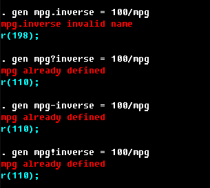
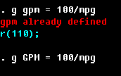
It is usually not a very good idea to create variables with names beginning with an underscore character, as Stata uses such names for its internal purposes. Also, it might be a good idea to develop your own system of naming conventions. This may come easy for some data sets that have very strict naming conventions, and it is easy to build on those. For instance, the data set from DHS have variable names v*, s* (various individual and household characteristics), b* (information on births), m*, h* (medical history of a child), so using names starting with say a (an added variable), d (derived characteristics) or x (what other name can you think of a variable???) would be a strong indication that those variables are not a part of the original data, but something that was created by the researcher.
Do you remember the discussion about accuracy? Well, here it is in action:
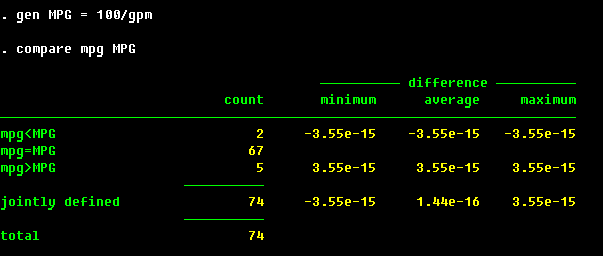
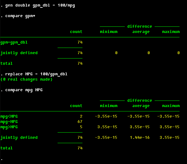
A good style of data handling implies that you have labels for all the
variables you create. Stata's way of handling labels is obviously with a label
command:
. label variable gpm "Gallons per 100 miles"
. lab var MPG "Mileage"
. lab var gpm_dbl "Gallons per 100 miles, double precision"
. lab var dome "Domestic car"
If there is something else you want to keep in mind about a variable, you can
add a little note to it:
. note MPG "Not the same as mpg although should be!!!"
You can also add notes to the whole data set:
. note "Toy data set I played with in my first Stata classes"
Try describe now to see how Stata signals the presence of notes.
See also UCLA Academic Technologies Services Stata website for more
on creating new variables and
on labels.
For a variable that has just few categories, one can set up a set of labels by another
incarnation of label:
If you are not happy with the name of the variable, you can easily rename it:
Stata has a special command to deal with changing the values of a categorical variable,
see recode.
Minor changes
Suppose you do not like some entries in your new variable, or you need to
create a new variable according to some complicated scheme. Then an additional
command you would need is replace. For instance, if you are not quite
sure about the fuel economy of the cars that don't have a repair record, you
may want to do this:
. replace mpg = . if mi(rep)
Suppose now you want to divide all cars into three groups according to the
level of the mpg variable. Here's one way to do this:
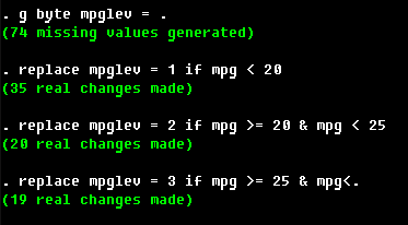
. g mpglev = 1 + (mpg >= 20) + (mpg>=25) if ~mi(mpg)
. lab var mpglev "Categorized mpg"
The if condition is probably excessive here as there are no missing
entries of mpg in the data set, but it is a good practice to keep track
of your missing observations, just in case. (A very telling joke about programmers
is that when a programmer goes to bed, he puts two glasses by his bed. He fills one with water,
in case he wants to drink during the night, and leaves the other empty, in case he does not
want to.) Other than that, it suffices to recall that logical expressions produce either
1 or 0 to see how this command works.
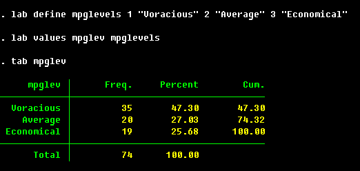
. lab define mpglevels 1 "Voracious" 2 "Average" 3 "Economical"
. lab values mpglev mpglevels
Those labels will be shown in tabulations:
. rename mpglev mpg_categorized
Functions
Stata has a large number of built-in functions. Take a minute (well... five minutes
or so) to browse through the whole list by whelp
function. Stata's functions can be used anywhere where you can fit exp
in the syntax diagram. The following may not make much sense per se but is a valid thing
to do in Stata:
. gen lweight = log(weight) if sin(trunk+round(gear,0.5) )>0
Self Check:
Generate the following variables and make appropriate labels:
|
Self Check:
Generate the following variables and make appropriate labels:
|
There are special commands to convert the missing values to number, and vice versa
(often, the missing data are denoted by numbers such as 99 or -1 in the raw data;
those would be read as such, and it will be your responsibility to convert them to
the missing data), mvencode to change missings to numbers, and mvdecode
to convert numbers to missing values. In principle, those are no very much different
from replace, but they would be making your code slightly more elegant and readable.
USE WITH CAUTION! Remember that they overwrite the existing data, so make sure
you can still recover what was missing.
For most of the "use with caution" operations, there is a relatively simple trick to
protect your data. First, you
See also UCLA ATS Stata website.
The second use might be to refer to the neighboring observations:
A third use might be to create something like a grid of points:
Subscripting is not to be mixed up with the range selection with the help of
in qualifier:
Uses of the by are way too numerous; see N. J. Cox, Speaking Stata:
How to move step by: step,
The Stata Journal, 2 (1), 86--102. Here's a few examples.
Let us stop here and review what we've done in this class:
On to the next class, to learn about Stata estimation
commands in general, and linear regression toolbox, in particular.
Questions, comments? E-mail me!.
Getting rid of stuff
There are two commands in Stata that eliminate unneeded observations or variables.
keep keeps the specified part of the data set, and drop deletes it
. keep make - foreign
returns your data to the original state, just as if you typed sysuse auto, clear.
To keep/drop specific observations, use if/in qualifiers:
. drop if mi(rep78)
USE WITH CAUTION! And make sure you still have all of the original data that
you need for your research.
. preserve
your data, and after you have completed some risky (in terms of the data loss) computations,
you can
. restore
your data from the preserved state. (Technically, Stata creates a temporary file
on disk and writes your data there, so if you have a few hundred megabytes of data, this will
take a while.)
Subscripting
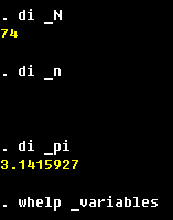
Stata has special quasi-variables that are always "present" in the data called
"underscore variables". The most important ones are the number pi denoted as
_pi, the current observation number _n and the total number of
observations _N:
. gen long obsno = _n
. lab var obsno "Observation ID"
. compress obsno
This sequence will create unique and valid IDs for a data set of any length.
This ID can be used for sorting when you want to keep the order of observations
after an ambiguous sort command:
. sort for obsno
will produce a well defined ordering by an important variable foreign
and an auxiliary variable obsno. It takes more computer time than
. sort for
but guarantees a unique ordering where it is relevant.
. gen dprice = price - price[_n-1]
. lab var dprice "Delta price"
. gen grid = (_n-1)/(_N-1)
. lab var grid "The grid between 0 and 1"
(self check: why the need to subtract 1?), although there is a somewhat more
explicit command range for this particular task.

by ... : construct
Stata has a smart and powerful way of performing operations on groups of observations.
Many Stata commands can be prefixed with
by varlist: ...
or
bysort varlist (sortlist) : ...
What Stata does with this construct is it breaks the data set into groups
identified by the unique combinations of the varlist variables and performs
the specified command on those subgroups. The bysort variant of that is to have
the observations sorted by sortlist within those observation groups.
The subscripting variables _n and _N indicate the current and the
last observations within the by-groups.
The difference between the by: construct and the by() option of some
commands like egen is that by: divides the data set into pieces in such a way
that Stata does not "feel" other parts of data when the command is run on a the current subsample.
The by() option, however, is specific to a command and may have different meanings to
different commands. See a note at
UCLA Academic Technologies Services Stata website demonstrating the use of by() option
in a simple two sample comparison.
. egen avgmpg = mean(mpg), by(foreign)
would be
. by foreign: gen avgmpg = sum(mpg)/_N
. by foreign: replace avgmpg = avgmpg[_N]
(self-check: make sure you understand how it works. Sketch the dataset with division
by groups, and see what Stata does on each step. Verify your argument with the above commands
and list-ing of the intermediate and final results.) Don't forget to label your
newly created variable!
. egen byte forXrep = group(foreign rep78), missing
would be
. bysort for rep: gen byte forXexp = 1 if _n == 1
. replace forXexp = sum(forXexp)
(self-check: make sure you understand how it works. Sketch the dataset with division
by groups, and see what Stata does on each step. Verify your argument with the above commands
and list-ing of the intermediate and final results.) Don't forget to label your
newly created variable! A word of caution: the group where any of the grouping variables is missing
is assigned a distinct value of forXexp. To overcome this efficiently, we would need
to know something about cycles (or simply omit the missing option in egen).
. bysort varlist: gen byte proper = (_N == 1)
If you want to check this for all variables in the data set, put * for the
varlist. In double-entry of data sets (when the results of a survey are typed
in by two coders independently), you would want to combine the data sets (more on that
later on the way) and see if all combinations of the relevant variables (except the coders'
IDs) are the same by the above command but with _N == 2 instead of _N == 1.
Stas Kolenikov